Supply chain management is a frequently encountered phrase these days, as managers strive to improve factory performance. The trouble is that all too often the real meaning is lost. Instead, a casual observer might interpret the activities at the factory as evidence of an intensive effort to improve supplier management.
Good supplier management, while praiseworthy, does not constitute good supply chain management without a concurrent effort to manage the rest of the aspects of delivering products to customers. In this article, I will present a complete supply chain management methodology. This approach, developed at Hewlett-Packard, will enable a manufacturing operation to better manage its supply chain, ultimately improving customer satisfaction levels while reducing overall costs.
Hewlett-Packard has successfully used this methodology and is making efforts to implement the practice of good supply chain management at all its divisions. HP identified the need to improve its process for manufacturing and delivering products to customers as profit margins suffered pressure from increasing competition. Other factors have contributed to a renewed focus, namely:
HP’s methodology has led to major changes in the way it does business. In the process, though, we have also discovered some appealing side effects. The proper execution of this methodology leads to improved team-work and cooperation among employees, especially those normally separated by either business function or geography. We’ve also discovered that this methodology leads to greatly improved customer focus, in addition to better relationships with suppliers.
In the following pages, I will introduce HP’s methodology. First, I will identify the problems inherent in supply chain management. Then, I will describe some key insights and briefly describe an analytical tool that we have developed to support a rational analysis of real supply chains. Finally, I will close with representative case studies describing HP successes with “real” supply chain management.
Large manufacturing companies are “hostage to complexity,” according to Lew Platt, HP’s president and CEO. The nature of the complexity is evident in a review of material flows for a complicated product. Multiple suppliers ship to manufacturing sites with varying regularity. There, subassemblies and final products are made by complicated and somewhat uncertain processes. Products are then shipped to direct customers, OEM customers, and “internal OEMs” (downstream manufacturing divisions of the same company treating the first factory’s “final” product as but one of their many component materials). The scene is further confused by the wealth of transportation options available: planes, trains, trucks, and ships. And, of course, multiple carriers convey products to customers spread across the globe. The permutations (most of which are actually used) defy proper management.
The real problem with such a confusing network is the uncertainty that plagues it. This uncertainty — observed on a daily basis as late deliveries, machine breakdowns, order cancellations, and the like — leads to increased inventories. In fact, inventory exists more or less as simple insurance against uncertainty. In the case of a single factory, this uncertainty, while bothersome and costly, is relatively easy to overcome with properly sized inventories of raw materials, work in process (WIP), and finished goods (FGI). Using simple statistical techniques, it’s straightforward to figure how much to hold so that, say, 95 percent of the time a customer will find in stock the product he or she wants, despite the uncertainties in the factory process.
However, the problem is much more complicated when one considers the whole network. Uncertainty propagates through a manufacturing network. Consider the following case: A supplier of raw silicon to an integrated circuit (IC) manufacturer delivers a bad lot. Without properly sized safety stocks to buffer the production line against such an event, the IC manufacturer in turn delays its deliveries to one of its customers, a computer manufacturer. The shortage of parts shuts down the computer line, and shipments to computer dealers across the country are late. A customer walking into his neighborhood computer store discovers the machine he wants is out of stock. However, the opportunistic salesperson sells him a competing machine available then and there. For want of an on-time silicon delivery (perhaps many months earlier), a sale is lost.
Now that’s an extreme example. Nearly every manufacturer carries some inventory to protect against such situations.1 The real difficulty is knowing how much to hold and where to hold it, for the propagation of intrinsic uncertainties is mathematically complicated. Because previously there was no clear, analytical way to calculate a proper inventory level (and because there was no clear insight into other processes in the supply chain), firms have traditionally relied on a combination of experience and intuition. This has been their only recourse against the vagaries of their supply chains.
In the face of increasing pressure to reduce inventories and simultaneously improve customer service, the different organizations in a supply chain find themselves working at cross-purposes. This is true when the organizations exist side by side within the same operation as well as when they are physically remote, independent companies.
What often happens is this: One organization will reduce its inventory to reduce cost. Typically such reductions hurt service. To build up service again, heightened pressure is put on suppliers (which might be the line running just across the aisle) to improve their performance. If this can be achieved only by increasing the supplier’s own inventory, the downstream operation’s inventory reductions might be completely canceled out. In many instances, a “broken” supply chain will have substantial stock held at one point to enable another node in the supply chain to skate by with minimal stock. Overall, there is too much stock held in the supply chain system. Reapportioning the stock would reduce the overall inventory investment and improve end-customer service levels. Unfortunately, most organizations are designed to create winners and losers; working together for system optimization receives little more than lip service.2
Only analytical techniques — or darned good luck —can precisely tune a supply chain. In our experience at HP, even the best-run supply chains could reduce their overall inventory investment by 25 percent by more cleverly distributing stock within their systems. More typically, 50 percent reductions are possible.3 With the proper tools, understanding and improvement will come from the following three steps:
When we first started investigating the problem of modeling Hewlett-Packard’s worldwide inventory networks, we found ourselves grappling with three fundamental questions. They stemmed from our interest in studying a difficult academic problem and from our desire to provide value to the company by providing appropriate solutions to real problems. First, could we develop a simple, generic framework to describe the supply chains we faced? Second, could we accurately model the propagation of uncertainty up and down the supply chain? Finally, could we create a modeling approach to support strategic decision makers and not simply provide yet another tool for solving day-to-day operational problems?
As our work progressed, we found that the answer was yes to each of the questions. What started as questions evolved into the three key elements of our work. They represent our greatest insights to the problem of managing supply chains. We repeatedly use a single, generic model to capture the salient features of each node in a supply chain. We carefully account for the upstream and downstream effect of uncertainty introduced at any node. And we answer questions posed by strategists, not tacticians.
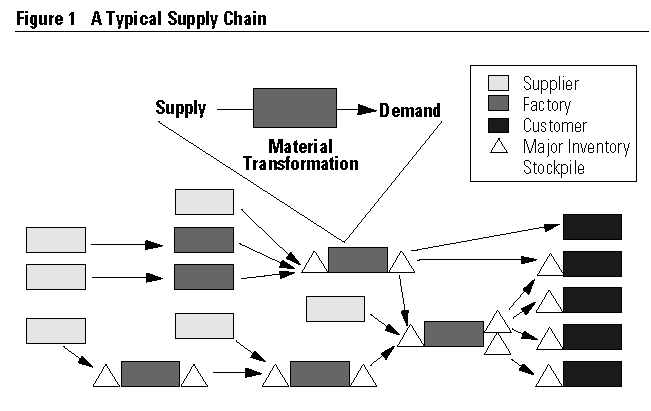
From an analytical point of view, a supply chain is simply a network of material processing cells with the following characteristics: supply, transformation, and demand (see Figure 1). This model applies at many levels. One can view a factory in this way just as easily as one can view an individual process step within that factory. In both cases, the central manufacturing process —whether it’s called “automobile assembly” or “spot-welding station 109a” — requires raw materials from some supplier external to the process. Those materials are then transformed in some manner that adds value, creating a stock of finished goods (though a JIT process might have an empty stockpile). Finally, there is demand from external customers for the goods produced. Because of the strategic nature of our work, we avoid diving too deeply into the internal workings of an individual factory.
An important aspect of our approach is that we model material handling and distribution functions in the same way as more traditional “manufacturing” processes. They follow the simple rule we apply: materials arrive, value is added, and products exit. In a warehouse, goods arrive in a truck or on a lift. The distribution team adds value by sorting the deliveries, breaking down pallets as needed, and racking the materials. The distribution operation then fills orders for those finished goods. That spot-welding station might even be one of the customers.
The reason we keep inventory is simple. Inventory is insurance — protection against life in an uncertain world. To meet our objectives for customer service, we keep a little extra material around (in what we call “safety stocks”) so that service won’t be adversely affected when something in the upstream process goes wrong. Understanding the impact of variability in the system is the goal of modern inventory control theory.
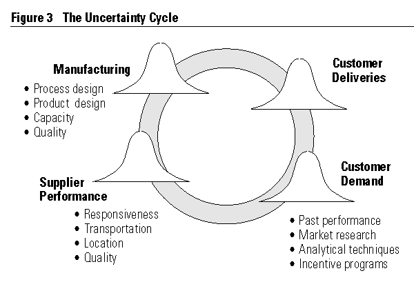
In fact, there are three distinct sources of uncertainty that plague supply chains: suppliers, manufacturing, and customers. To understand fully the impact on customer service and to be able to improve performance, it is essential that each of these be measured and addressed. The systemwide impact of each source of uncertainty must also be understood. Figure 2 illustrates how the three sources of uncertainty in the system combine to affect deliveries to customers.4
The first source of variability that leads to holding safety stocks is supplier performance. This is where naive supply chain considerations start and end. Your supplier quotes a lead time, but — alas! — he has a hard time getting you his materials exactly when he says he will. A storm delayed a delivery. A machine broke down. One of his suppliers was late. Any number of things could account for the late delivery, but in the end, it remains that sometimes those shipments are late (and, of course, sometimes they’re early).
Over time, the vagaries of each supplier’s delivery performance can be tracked. Each supplier’s on-time performance, average lateness when late, and degree of inconsistency (as measured by the standard deviation of lateness) are the data to maintain. These data are immensely valuable, for the characteristics of each supplier tell you how much extra stock you must hold to keep your line up and running reliably. Supplier performance — and the factory’s response, in the form of safety stocks — help determine downstream customer service.
The second source of variability comes in the manufacturing process itself. Here, a host of familiar problems can stop the flow of materials off the end of the line. Machines can break down (just as they can for your supplier), another project can tie up a key worker, or a computer foul-up can route materials to the wrong place.
In measuring process performance as it applies to overall supply chain performance, the key metrics are frequency of downtime (for the entire process, not just this or that machine), repair time, and the variation in the repair time. Note that again we’re focused on a probability distribution of performance, for that is the nature of uncertainty. Sometimes the line runs for a week without shutting down. Other times, it seems we can’t keep it running for more than an hour or two without a major shutdown. The reliability of the process — or its lack of reliability — is one of the three principal determinants of downstream customer service and the inventory investment to achieve that service.
Customer demand marks the third and final major source of uncertainty in the supply chain. Depending on the factory’s location in the supply chain, this may reflect irregular purchases by a fickle public. Or it may stem from irregular orders from an industrial customer responding to its own up-and-down demand.5 In any event, true build-to-order factories are relatively rare, and most factories keep some stock, filling orders from inventory as needed. The more variable the orders, the more stock required to reliably meet customer demand. Knowing average demand and the variability of that demand makes setting inventory goals more scientific and less seat-of-the-pants.
Unfortunately, week-to-week demand variability is often not the only problem. Because of long lead times, factories build stock in an attempt to meet forecast demand. Hewlett-Packard, for instance, often contracts for raw materials eight months or more before the final product will reach finished goods inventory. Thus, customer service in August depends on HP’s ability to anticipate demand the preceding January. The effective variability in this case is greatly compounded from the actual variability we will experience come August.
We can measure historical order performance and attempt to use that information to predict future orders. Market research can help too. But such a strategy is often little more than a shot in the dark when introducing a new product. With ever-shortening product life cycles, our exposure to this final element of variability in the supply chain occurs more frequently.
Customer service starts and ends with the customer. The customer feels the full effect of the complex, interacting uncertainties in the supply chain. In Figure 3, we show what we’ve coined as the “uncertainty cycle” to capture this effect. The forecast — based on historical customer behavior — starts things rolling. Materials are purchased and delivered by suppliers. Then the factory takes its turn, producing the finished goods. Finally, the early forecasts are realized in the form of hard orders, and products are shipped to customers. This cycle repeats itself up and down the supply chain. It also repeats over time.
Strategic initiatives can lessen the impact of uncertainty. First, we can reduce the uncertainties using a standard total quality control approach. We can improve forecast accuracy through advanced analytical techniques.6 We can investigate more reliable transportation modes. We can encourage suppliers to perform more reliably.7 And we can change product designs to stabilize manufacturing processes. The costs associated with these changes can be balanced against the savings of reduced supply chain inventories or improved customer service.
Unfortunately, we cannot reduce all uncertainties. But other initiatives can redesign the supply chain to reduce the impact of the uncertainties. For example, opening a new factory can put production closer to key customers. I’ll return to this point shortly with some specific examples from HP’s experience.
A sound supply chain modeling methodology can address long-term problems. Focusing on the uncertainties in the system and the way they propagate up and down the chain can lead to new operating policies and objectives. Using tactical tools like transportation models, scheduling algorithms, or fast MRP programs can fine-tune the performance of the system.8
At HP, we have developed a decision support system that allows us to model supply chains analytically. The tool captures the spirit of the model characteristics described above, though the mathematical details are not appropriate for this discussion.9 As we explain to our internal HP customers, the tool is of little value unless one grasps the underlying methodology of supply chain modeling. Supply chain performance can be improved substantially without even switching on a computer. Nonetheless, there are a few points related to the use of the analytical tool that are important.
As noted earlier, there are many performance measures, like supplier lateness and the associated variability, required to adequately model a supply chain. Ideally, this data would be collected routinely. After all, these are fundamental measures. However, we have yet to work with an organization that has the data readily available.
While organizations typically imagine they can collect the necessary data within just a few weeks, it invariably takes six months or longer. Perhaps the single greatest reason for this is that businesses have not taken a careful look at uncertainty in their operations. This is a major failing on their part. Not only have they been ignoring one of the critical drivers of their performance, they force themselves to wait while collecting enough data points to ensure an accurate representation.
Another common problem with collecting the right data stems from the breadth of the supply chain itself. Because the typical supply chain comprises many organizations, data must come from many disparate locations. To ensure success of the modeling effort, it is necessary to obtain sufficient commitment of resources to ensure accurate, useful data about each of the links in the supply chain. Even within a single site, cross-functional cooperation is necessary.
Accuracy of the available data can present a problem too. Often the collected data paints a false image of an operation due to data entry errors, inconsistent collection procedures, and system incompatibilities. The breadth of the supply chain can compound the accuracy problem, for two sites often define their terms somewhat differently. A consistent, careful approach is needed in collecting data on the supply chain.
Finally, the collected data must be valid. Usually, some degree of abstraction is necessary. For example, it would be unwieldy to include every stock-keeping unit in a model that is used for strategic purposes only. Thus, some parts may be left out of the model completely (e.g., common nuts and bolts or passive electronic components). Others may be aggregated and represented in the model as a single, “generic” component, like “mechanisms.” The summarized characteristics of the aggregated parts must be checked against expert opinion to see if they represent the situation fairly. We often use the “worst case” to get a conservative model.
Usually, managers propose changes in operating policy and then carefully tally the costs of implementing the changes. However, even the best ideas often rot on the vine because of the difficulties inherent in quantifying the benefits associated with change. That is, typical decision criteria like net present value are not easily calculated; advocates are forced to rely on persuasive, qualitative arguments.
The tool we use at HP measures the benefits (or costs) of changes in supply chain policy. This fills a gaping hole in the strategic planning process. Specifically, our tool can tell the inventory requirements of a given supply chain, given the appropriate operating conditions and customer service objectives. Uncertainties throughout the supply chain are accounted for, and stockpiles are sized and valued accordingly.
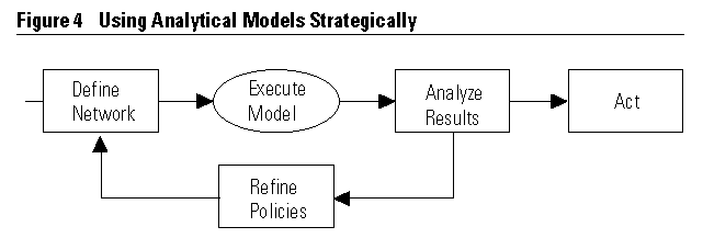
We use our analysis tool in an iterative manner, as depicted in Figure 4. The process allows us to investigate numerous possible changes before the fact and explore thoroughly the strengths and weaknesses of each. The insight we gain from one analysis can lead to refinements in the next. In many ways, our analysis is akin to the use of CAD/CAM software in a product design lab. Simulation detects many flaws before the expense of a physical prototype.
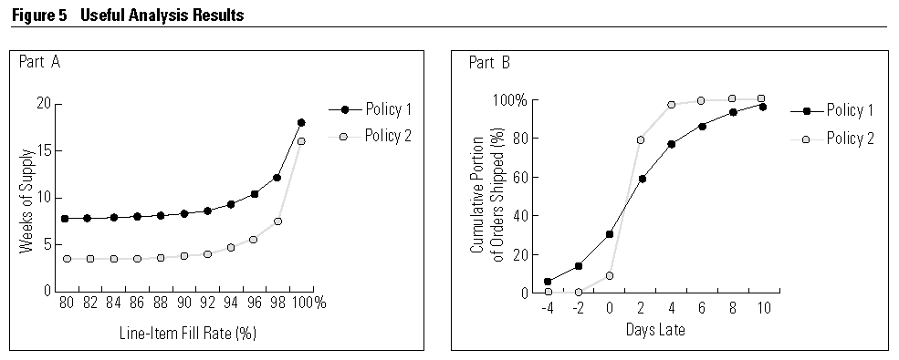
It is important that any analysis tool provide information to facilitate decision making. That is, the product of the analysis must be useful. We look at a number of factors when reviewing the output of our supply chain models. However, we remain focused on balancing cost and customer service. Examples of output that we find most useful are shown in Figure 5.
We use two key measures of customer service. For off-the-shelf items, the line-item fill rate is usually appropriate. This measures the fraction of demands filled immediately. On average, the more inventory kept on hand, the higher the achieved fill rate. That explains the general shape of the curve in part A in Figure 5. Two different policies — two alternative means of shipping products from the factory to the distribution center, for example — can lead to different cost/service curves. Policy 2, in this example, provides equivalent service at a lower inventory cost than Policy 1. The question remains, of course, whether the cost of implementing Policy 2 exceeds the anticipated benefits.
The second measure we use is the so-called order aging curve in part B in Figure 5. This describes the more general situation by looking not only at off-the-shelf performance but also at the likely delay if delivery is not immediate. It might be helpful to think of a build-to-order environment. In the case illustrated here, Policy 1 has the higher proportion of on-time deliveries (0 days late), but late orders may linger on the books for weeks. Implementing Policy 2 would lead to slightly diminished off-the-shelf delivery, but the bulk of all orders should be filled promptly. Policy 2 inflicts less variability on the downstream customer. In real terms, Policy 1 might represent the case of a factory with quite a bit of FGI, but unreliable suppliers. Policy 2, in contrast, sees less reliance on FGI but more dependable suppliers or sufficient stocks of raw materials to compensate.
It is crucial to interpret properly analysis results like those shown in Figure 5. The mathematics of inventory management theory focus on long-term, average performance — yet an individual order can only be early, on time, or late. Just as factories experience variations in supplier performance or process uptime, there will be periods where customer service is high and other periods where it is low. The key is that the analytical curve represents an “efficient frontier” — the best possible performance given the operating characteristics. While it is possible to perform worse than the curves (i.e., results above the line-item fill-rate curve), better performance is impossible over an extended time. Thus, the curves presented as examples suggest average performance over the long haul, a goal to strive for. As they say, “your mileage may vary.”
Despite a theoretical nature, output such as this is useful. Often performance is not adequately measured in these ways. Especially lacking is historical data on the variability of delivery performance. Simply discussing new ways of measuring performance — and the reasons for setting different performance targets — can lead to improvements in overall supply chain performance.
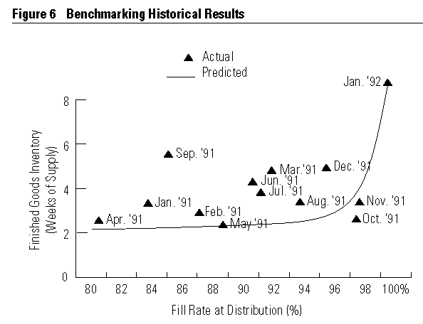
Benchmarking with data on historical performance is important to validate the results. If the model doesn’t reflect reality, then it is dangerous to suggest its use to facilitate decision making. On the other hand, once validated, the model can be used with confidence on extensions from the base case. In the supply chain arena, we generally plot performance on a monthly basis. The goal is to match as closely as possible the predictions of the analytical model, as they do in Figure 6.
So how can there be points below the curve? Doesn’t that curve define the minimum required inventory to meet customer performance goals? Yet Figure 6 shows that in October 1991, the service level was 98 percent with two and a half weeks of inventory. Theoretically it would take four weeks of inventory to achieve that level of performance; two and a half weeks buys you only 92 percent. The explanation gets back to the matter of long-term averages. Generally, a site holds too much inventory, and just as we see in Figure 6, most of the actual results fall well above the theoretical curve. Operational difficulties of one sort or another explain why performance strays from the theoretical. Exceptionally high orders, for example, might lead to a stock out situation and poor customer service results. A slow order month, though, will lead to good results. The usual amount of inventory leads to higher than average fill rates simply because there were fewer customers than usual.
I have described a framework for modeling supply chains in the preceding pages. But what good is it? Next I’ll describe a few cases of the successful application of this modeling approach. The first is about the manufacture and distribution of one of Hewlett-Packard’s most successful products, the DeskJet family of thermal ink-jet printers. The second case describes the situation HP faced when considering a new, cooperative manufacturing venture with an Asian partner. In the final case, I present some results that clearly indicate directions for future work in this area.
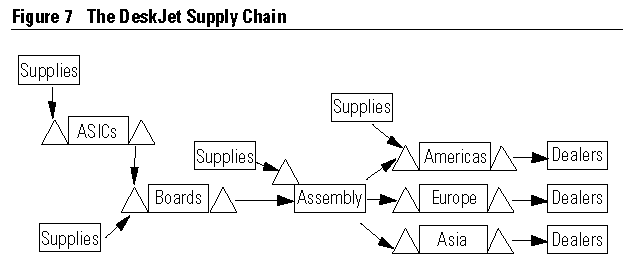
The supply chain for the DeskJet family of low-cost printers has five physically separate Hewlett-Packard facilities that contribute to the manufacture and distribution of the printers; the same shop assembles printed circuit boards and completes printer assemblies (see Figure 7). The pipeline itself is nearly six months long.
The product managers wanted to reduce their susceptibility to variability in the supply chain. Under then-current policies, they had to keep excessive amounts of inventory, and that tied up cash they might otherwise have applied to other projects. The division met its customer service goals, but the managers felt that there must be a way to lower costs without sacrificing customer goodwill.
Under the existing policy, the factory “localized” products. That is, the central factory manufactured and packaged printers for each of the local markets served, adding a power cord and transformer to meet the plug and voltage needs of the country and a manual written in the proper language. The result was that the factory produced over a dozen variations of each seemingly identical printer. Each distribution center kept on hand a substantial stockpile of each printer/country option to fill the erratic pattern of orders received. This was especially troublesome in Europe, where there are more options produced for relatively small markets (e.g., Denmark).
The safety stocks required to meet high service targets were huge. Because the division chose to segregate the total market into its constituent components, it subjected itself to heightened variability — orders for Danish printers are much more unpredictable than the overall demand for printers in Europe. The question quickly became: What would be the value of risk pooling? Localization could be postponed to the distribution step; the factory could ship generic printers. The distributor would then combine the printers with the proper manuals and power cords only after receiving firm orders. This would greatly reduce the total safety stock (of generic printers).
We modeled the DeskJet supply chain to determine by how much switching to a generic printer would reduce the inventory investment. The results, shown in Figure 8, persuaded the distribution center to accept the plan. Under the old policy, and with a service goal of 98 percent, roughly seven weeks of FGI were required. Changing to a generic printer strategy would reduce the inventory requirement to about five weeks. The savings — worth over $30 million a year at current volumes —come from postponing the commitment of the generic printer to a specific model. Also contributing to the savings is the fact that stocks of generic printers are less valuable than a stock of an equal number of localized printers. That localization step adds value. Finally, the savings are not as great at lower service levels. High off-the-shelf service rates are relatively expensive.
The savings from the reduced inventory (valued at a relatively high cost of capital because of the risk of write-offs due to short product life cycles) more than compensated for the cost of implementing the changes. Increased supplies of localization materials are necessary when postponing localization to distribution, but those costs are relatively small. The icing on the cake? Shipping costs dropped by several million dollars a year because shippers can pack generic printers more densely in bulk.10
Generic printers localized at distribution centers make sense in regions where there are many printer options. However, adding the manual and power cord is a slightly more expensive proposition at the distribution center than at the factory. This was a particular concern in the United States, where inventory savings for a generic printer are small, since virtually all U.S. volume is for the same model. An extension of the DeskJet study investigated the possibility of producing two printers at the factory — an ultra-low-cost unit destined exclusively for the U.S. market and a generic printer to serve the rest of the world.
Weighed against unit cost savings with this U.S.-only model was this supply chain consideration: with 100 percent generic printers, stockout conditions could be quickly remedied using a lateral re-supply mechanism. If orders for a generic printer in Europe exceeded demand, the U.S. or Asia/Pacific distribution centers could send emergency shipments of the same printer in just a few days and restore high customer service quickly with little expense beyond air freight costs. With factory-localized printers, there would be expensive rework at the distribution centers too. The distributor would have to open a sealed box, change the cord and manual, and fill a new box. Labor and material costs would go up.
Under routine business conditions, this may not seem like a tremendous potential saving. However, consider the scenario of a new product introduction. Initial forecasts are for a lukewarm reception in Europe, while everyone expects the printer to be a big hit when introduced in the United States. We fill the pipeline accordingly. Then, against all odds, the forecasts prove to be exactly backward. Although having accurately projected worldwide demand, HP faces the unpleasant predicament of having orders it can’t fill in Europe while the U.S. distribution center is stacked to the rafters with excess printers. With a generic printer strategy, those slow-moving printers could be immediately shipped to Europe. The alternative would be to wait and slowly let new production fill the pipeline to the European customers. With windows of opportunity for new products growing ever smaller, the ability to design the supply chain to protect against such unexpected circumstances is quite appealing.
As product life cycles shorten, Hewlett-Packard is facing more and more situations like this. The value of considering the problem in advance and devising a strategy using a supply chain methodology measures in the millions of dollars. In this case, generic printers reduce HP’s exposure to forecast uncertainty. And when things do go wrong, they make recovery swifter and less costly, without sacrificing customer service.
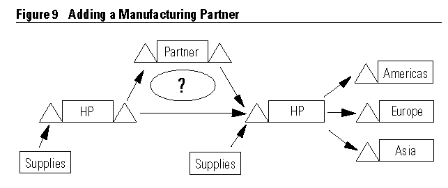
In another Hewlett-Packard business, one of the factories had the opportunity to form a joint venture with a low-cost Asian manufacturing partner. This new partner would add an intermediate process step between two HP plants in lieu of a process handled at HP (see Figure 9). The perceived drawback was that shipping to and from the partner would take a month on a boat. Including the partner’s processing time, the product lead time would increase by over three months!
The question was straightforward: How much additional stock would the distribution centers need if we added this intermediate step? At the time, the stock level was just over a month’s supply of FGI in the U.S. distribution centers.
The result was staggering. With no other changes to the system, nearly five months worth of FGI would be necessary to maintain the same service level as before, far more than initially anticipated. The increase stemmed from the increased product lead time. Demand was anticipated to be quite variable. Introducing a three-month lag in the middle of the process greatly increased the product’s exposure to changes in the marketplace.
These results opened our eyes to the value of rigorous supply chain analysis. While everyone involved knew that inventories would have to grow, we would have faced a terrible product shortage if we’d gone with our initial guesses. Moreover, the inventory situation forced us to take another look at our suitor’s proposed financial arrangements.
We proposed several alternative supply chains. Since both firms had production facilities in Singapore, the most attractive called for colocating the two firms’ factories. Doing all the work in the same place would virtually eliminate the onerous three-month delay, which was largely caused by shipping time. Our analysis gave us firm footing for negotiating a more attractive deal with our new partner. These results made the managers involved realize the importance of inventory in their decision-making process.
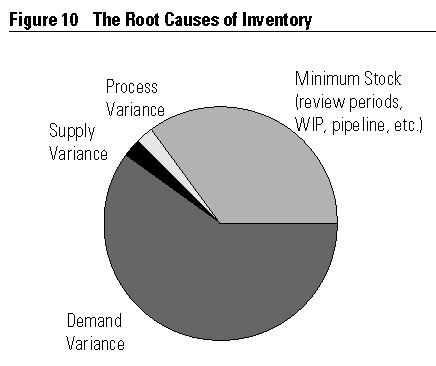
Studying various Hewlett-Packard supply chains leads to some startling conclusions. As we gain experience treating the supply chains as systems, we build insight into their nature. However, the results shown in Figure 10 are downright unnerving.
These results come from a single HP division, but follow-on work shows that the figure represents the rest of the business as well. We have categorized the total supply chain inventory by its cause or source. Naturally, any supply chain has a certain amount of essential inventory. This stock satisfies the so-called conservation of mass laws. There is work in process in the factories and products in the pipeline from site to site. Also, periodic review systems lead naturally to a certain average stock on hand, even if there is no uncertainty in the system. At HP, these “natural” stocks make up about 40 percent of the total inventory investment.
The three sources of variability account for the balance of the stock. In HP factories and at the corporate level, we have exerted tremendous pressure on suppliers to improve their performance. Only a small percentage of the total stocks stems from late deliveries, etc. That is, if all deliveries arrived exactly when expected, HP’s total inventory needs would drop just a few percentage points.
The same is true in manufacturing. HP processes are well-tuned. Moreover, the duration of process interruptions is negligibly short compared to the overall length of the supply chain. Thus, while a line may shut down fairly often for one reason or another, the global impact (from an inventory point of view) is not great.
The chief culprit is demand uncertainty. Over half of HP’s inventories are protection against irregular orders. There are two partial explanations for this: First, demand is truly variable. No one can anticipate just when a big order might come in. Similarly, we have a difficult time anticipating just what price point will trigger a sales rush. This problem is partly natural, but improved forecasting ability would help alleviate the problem. If we knew better what total month-to-month demand would be (a forecasting problem), it would be much easier to meet the day-to-day changes in order volume (a true demand problem).
Second, we set high customer service goals. For example, for our computer peripheral products, we commonly shoot for an off-the-shelf line-item fill rate in the three sigma range. That is, we hope nearly all our customers will have their orders filled immediately. Much stock is necessary to protect against those rare instances when demand is very high. We don’t always meet our goals, but operational problems or gross forecasting errors usually explain situations when we don’t. New product introduction and the unanticipated popularity of some products has led to allocation of insufficient supplies.
Historically, we have spent large sums honing manufacturing processes and working with suppliers. However, in a supply chain perspective, the big reductions in inventory expense in the future will come from improving HP’s ability to forecast demand and from designing products that allow better risk pooling. Continued efforts to improve product and process designs will reduce vulnerability to demand uncertainty, as with the DeskJet printer.
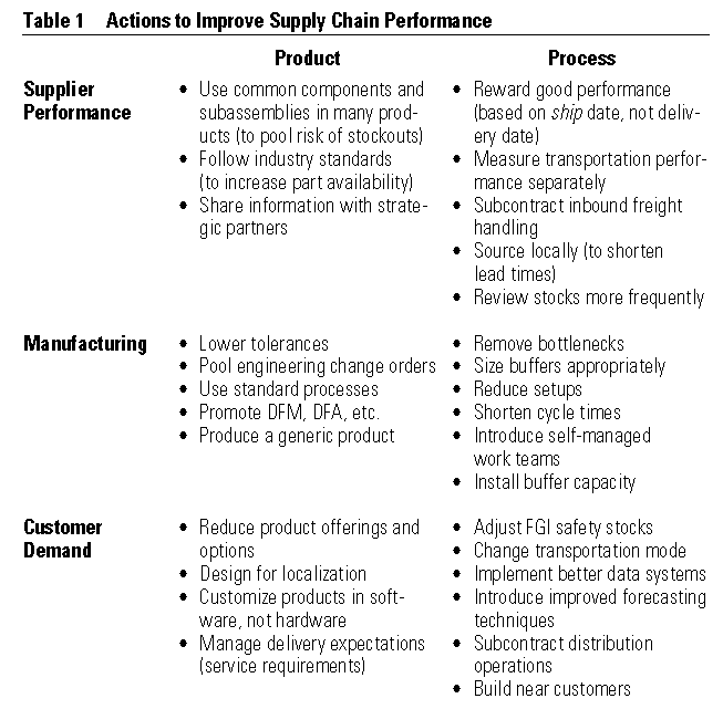
Sound data combined with the right quantitative techniques make thorough supply chain analysis possible. Without them, product managers must resort to qualitative approaches. Fortunately, there is a wealth of opportunity in most supply chains, even if using a simple, commonsense approach. Managers can implement a few obvious changes and best practices while collecting the first solid data on supply chain uncertainty. Then, once the data is available, they can fine-tune the system using a rigorous, analytical approach.
Table 1 outlines some of the ways to reduce or avoid uncertainty in the supply chain. Changes to product and process will stimulate reductions in the uncertainties plaguing each node in a supply chain, namely, supplier performance, manufacturing, and customer demand. These actions are not without costs.
The value of taking a systems view of the problem cannot be overstated. Organizational barriers introduce tremendous inefficiencies in supply chains. It is critical that all players in the business of getting products to customers consider their role in the objective of satisfying the customer. Strategic decisions on supply chain design can increase customer satisfaction and save money at the same time — the classic win-win situation.
Clearly, supply chain management should not be confused with supplier management. Supply chain management covers a far broader scope. Approaching problems with a systems view and a sound supply chain methodology can lead to great savings. At Hewlett-Packard, we have little doubt that hundreds of millions of dollars lie in the balance. Judging from our discussions with suppliers and customers, the same is true for other firms.
ABOUT THE AUTHOR
Tom Davis is a process technology manager at Hewlett-Packard.
REFERENCES (21)
1. Even JIT fanatics carry inventory of finished goods close to the customer and with suppliers. These stockpiles are small, though, because the manufacturing process has been tuned (1) to reduce uncertainty in the first place and (2) to recover quickly when something does happen. Paul Zipkin describes this as “pragmatic JIT.” See:
P. Zipkin, “Does Manufacturing Need a JIT Revolution?” Harvard Business Review, January–February 1991, pp. 40–50.
Show All References
ACKNOWLEDGMENTS
The author is grateful to his coworkers on HP’s Strategic Planning and Modeling team for their contributions: Corey Billington, Rob Hall, and Steve Rockhold; to Brent Carter from HP’s Vancouver Division; and to Hau Lee of Stanford University.
Chat with us on WhatsApp
 UK Registered Office
UK Operational Office
UK Registered Office
UK Operational Office
 Bangladesh Contact Office
 Malaysia Contact Office
 Ghana (Accra) Contact Office
Ghana (Eastern Region) Contact Office
Ghana (Accra) Contact Office
Ghana (Eastern Region) Contact Office
 Tanzania Contact Office
 Nigeria Contact Office
 Kenya Contact office
 Philippines Contact office